Optimizing Server-Side Rendering for Billion Plus Row Datasets

MapD was built from the ground up to enable fully interactive querying and visualization on multi-billion row datasets. An important feature of our system is the ability to visualize large results sets, regardless of their cardinality. Ordinary BI systems do fine when rendering standard bar or pie charts but often fall over when required to render the millions of records often associated with scatter plots, network graphs and various forms of geovisualization. Being able to visualize large numbers of records at the grain-level in near real-time is critical for giving an analyst a “full view” of their data, resulting in better analytical outcomes.

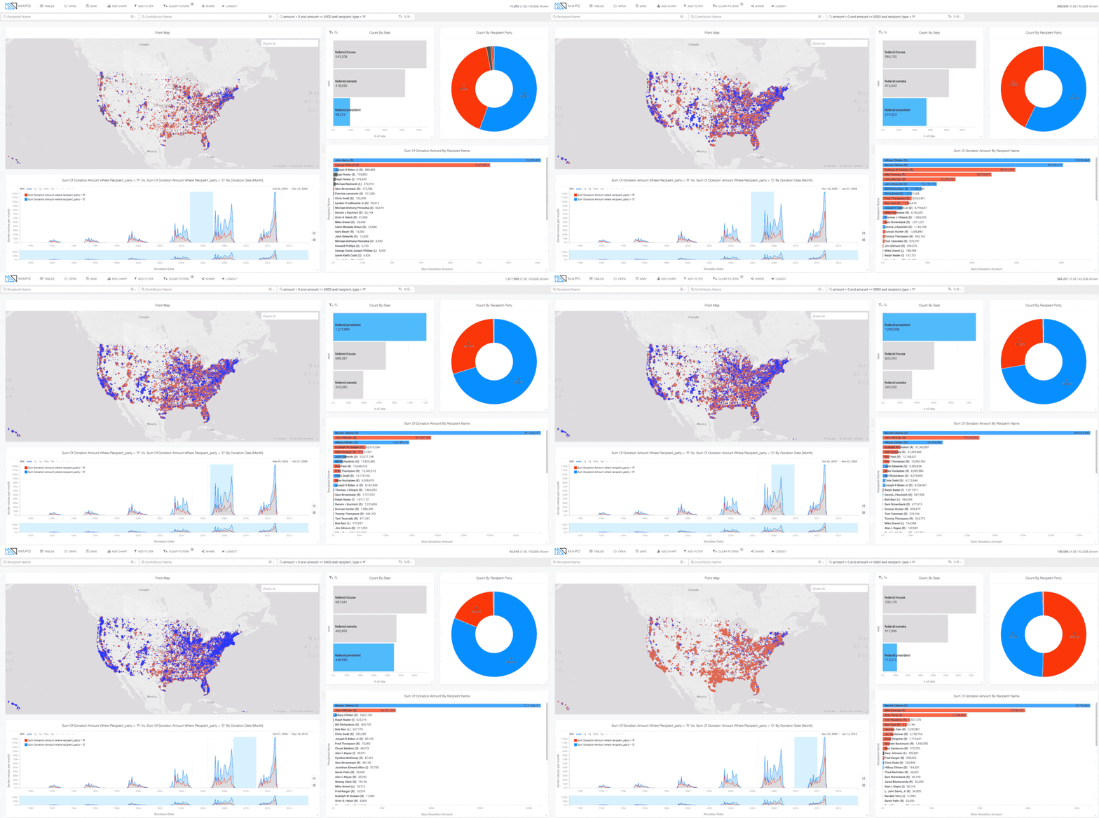
Figure 1: Data from over 28 million political donations. Basemap courtesy of © Mapbox © OpenStreetMap

The desire for real-time interactivity presented several design challenges to our stack:

1. Would server or browser be responsible for rendering the visualization
2. How would we configure the visualization’s rendering properties knowing that many of them would need to be data-driven
3. Can the visualization be rendered in near real time

The Choice Between Frontend and Backend Rendering

At first glance it seemed like a logical choice to do all of the rendering in our web-based frontend. The advancements in WebGL in recent years has opened doors for heavier client-side rendering, and utilizing it would allow the server to focus solely on database operations.

Upon further inspection, however, this front-end approach held several significant drawbacks.

First of all, WebGL, even the recently released 2.0 spec, is missing a lot of useful functionality for optimal rendering compared with recent OpenGL releases (geometry/compute shaders, indirect drawing commands, and a variety of buffer objects like pbos and shader storage blocks to name a few). Furthermore, we would have to provide fallbacks in browsers where WebGL is unsupported.

Secondly, and more importantly from our speed-first perspective, network bandwidth is a bottleneck for the size of uncompressed data that might be required for certain visualizations. That could derail attempts at real-time interactivity.

These drawbacks led us to consider rendering on the backend as an alternative. As we discovered, this approach held several distinct advantages.

First of all, large datasets could be rendered and then rasterized on the server, reducing the data needing to be sent over the wire to common compressed images/video streams. Even when rendering only a few million points, sending the raw data over the wire to the client for the x, y, color and size channels can consume tens to hundreds of megabytes, while a compressed PNG might be weigh in at less than a hundred kilobytes.

Secondly, and even more importantly, we could take advantage of the native graphics pipelines of GPUs and use the CUDA/GL interoperability API to map GL buffers to CUDA space for an optimal query-to-render pipeline. In fact, these buffers fit into our query system so naturally that results could be rendered directly without any additional copy or reduction operations. This would prove integral for high frame rates.

Because we didn't want to burden the backend with a full featured render engine, we adopted a hybrid approach to the problem, leveraging functionality from both the frontend and the backend. For example, basic chart visualizations that required minimal data are rendered on the frontend by D3 and other common visualization toolkits.

On the other hand, we use OpenGL on the server-side to render visualizations such as pointmaps which can involve millions of points, passing the result to the frontend client as a PNG. We can then overlay these rendered images on a base map rendered using MapBox GL. Their low-latency, resolution-independent, vector tile format keeps network demands to a minimum and delivers near-instant rendering performance. Further, their effective rendering-API included a hook for adding custom layers to their maps making compositing our backend-rendered imagery a breeze.

The result was a hybrid system that delivered a lightweight and efficient frontend, and an optimized and load-balanced backend.

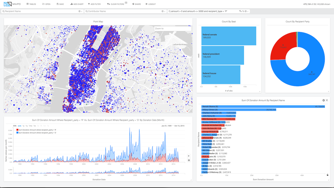
Figure 2: 25 years of political giving data in the NYC metropolitan area. Visualization dashboard includes D3 charts and a backend-rendered pointmap composited atop a MapBox JS map. Basemap courtesy of © Mapbox © OpenStreetMap.

The Data is in the Details

The backend can render data in a variety of different primitives including points, lines, and polygons, the properties of which can be linked to specific columns in the query result set and mapped to a preferred output via a library of scaling functions performed in the shader. We developed a JSON schema for declaring these mappings modeled after the visualization grammar format Vega developed by Dr. Jeffrey Heer, one of MapD’s advisors, and students of the Interactive Data Lab at the University of Washington.

Let’s look at an example.

Let’s say we have a large dataset of tweets which includes columns of the mercator-projected latitude and longitude GPS coordinates of the tweet named MERCX & MERCY respectively. We can run a simple projection SQL query to get at those coordinates:

{
"width" : 1024,  // image width
"height" : 1024, // image height
"data": [  // declare the data via sql
    {
        "name" : "tweets", // name of the data for referencing
        “dbTableName” : “tweets”, // name of the data table in the db
        “sql” : “SELECT MERC_X as x, MERC_Y as y FROM tweets;”
    }
],
"marks" : [ // now describe the render layers
    {
        "type" : "points",  // render as points
        "from" : {"data" : "tweets"},  // specify the data to reference
        "properties" : {
            "x" : {  // point x coord references x (or MERC_X) in the data
                "field" : "x"
            },
            "y" : {  // point y coord references y (or MERC_Y) in the data
                "field" : "y"
            },
            "fillColor" : “red”, // draw points red
            "size" : 10  // points will be 10 pixels in diameter
        }
    }
]
}

Although this description will work without error, it has some problems. First, you likely wouldn’t see any points in the final image since the position of the points are in mercator coordinates and not pixel coordinates. We have to specify a transformation from mercator space to pixel space.

We can do this simply with a linear scale in the JSON:

{
"width" : 1024,  // image width
"height" : 1024, // image height
"data": [...],
“scales” : [  // specify an x/y scale that will linearly map from 
              // mercator space to the image’s width/height
    {  
        "name" : "x",
        "type" : "linear",
        "domain" : [-20037508.3428, 20037508.3428], // MERC_X min/max
        "range" : "width"
    },
    {
        "name" : "y",
        "type" : "linear",
        "domain" : [-15496570.7397, 18764656.2314],  // MERC_Y min/max
        "range" : "height"
    },
], 
"marks" : [
    {
        ...
            "x" : {
                “scale” : “x”,  // scale MERC_X to pixel coords
                "field" : "x"
            },
            "y" : {
                “scale” : “y”,  // scale MERC_Y to pixel coords
                "field" : "y"
            },
        ...
    }
]
}

We will now see rendered points, but if the dataset has billions of tweets, this will be incredibly wasteful and would likely not render at all. Rendering billions of points will likely just flood OpenGL’s command queue to the point of failure or it would fill the image with so many points that you wouldn’t be able to decipher anything from the rendered result. In this case we are better off limiting the number of rendered points for both efficiency and clarity. We can do that in the SQL by adding a limit, let’s say 2 million points, while using a sampling method such as Knuth’s Multiplicative Hash to randomly select rows (the modulo component of the SQL query below).

SELECT MERC_X as x, MERC_Y as y FROM tweets WHERE MOD(tweets_nov_feb.rowid * 265445761, 4294967296) < 238780933 LIMIT 2000000;

The result of such a query limit will be a reasonable representation of the full dataset - other sampling methods could be used if desired.

Now let’s say we wanted to zoom in on tweets from the contiguous United States.

If we know the mercator bounds of the contiguous states to be (-13847031.458089568, -7451726.7126439) in X and (2664853.9336479248,6651537.411326187) in Y, we can add a filter to the SQL query to only return the tweets located inside those bounds:

SELECT MERC_X as x, MERC_Y as y FROM tweets WHERE MOD(tweets_nov_feb.rowid * 265445761, 4294967296) < 238780933 LIMIT 2000000;

Then adjust the mercator-to-pixel space transformation in the JSON with the same bounds:

 {  
        "name" : "x",
        "type" : "linear",
        "domain" : [-13847031.458089568, -7451726.7126439],
        "range" : "width"
    },
    {
        "name" : "y",
        "type" : "linear",
        "domain" : [2664853.9336479248,6651537.411326187],
        "range" : "height"
    },

Our renderer supports not just linear scales, but also quantize and ordinal scaling routines. This enables the user to map data-driven render properties to reasonable ranges of values.

For example, let’s say that our tweet dataset included a column describing the origin of the tweet (iOS, Android, etc.), let’s call it ORIGIN. We can get at that data via SQL:

SELECT MERC_X as x, MERC_Y as y, ORIGIN as orig FROM tweets LIMIT 2000000;

Now we can use ORIGIN to drive the color of the points using an ordinal scale:

 “scales” : [
    {  
        "name" : "color",
        "type" : "ordinal",
        "domain" : [“iOS”, “Android”], // the languages
        "range" : [“blue”, “green”],  // the color per origin type
        “default” : “yellow”  // set a default, just in case
    },
    …
]
…
“Marks” : [
         {
        "type" : "points",
        ...
            "fillColor" : {    // color the points according to language
                “scale” : “color”,
                “field” : “orig”
            }
        ...
    }
]

‍

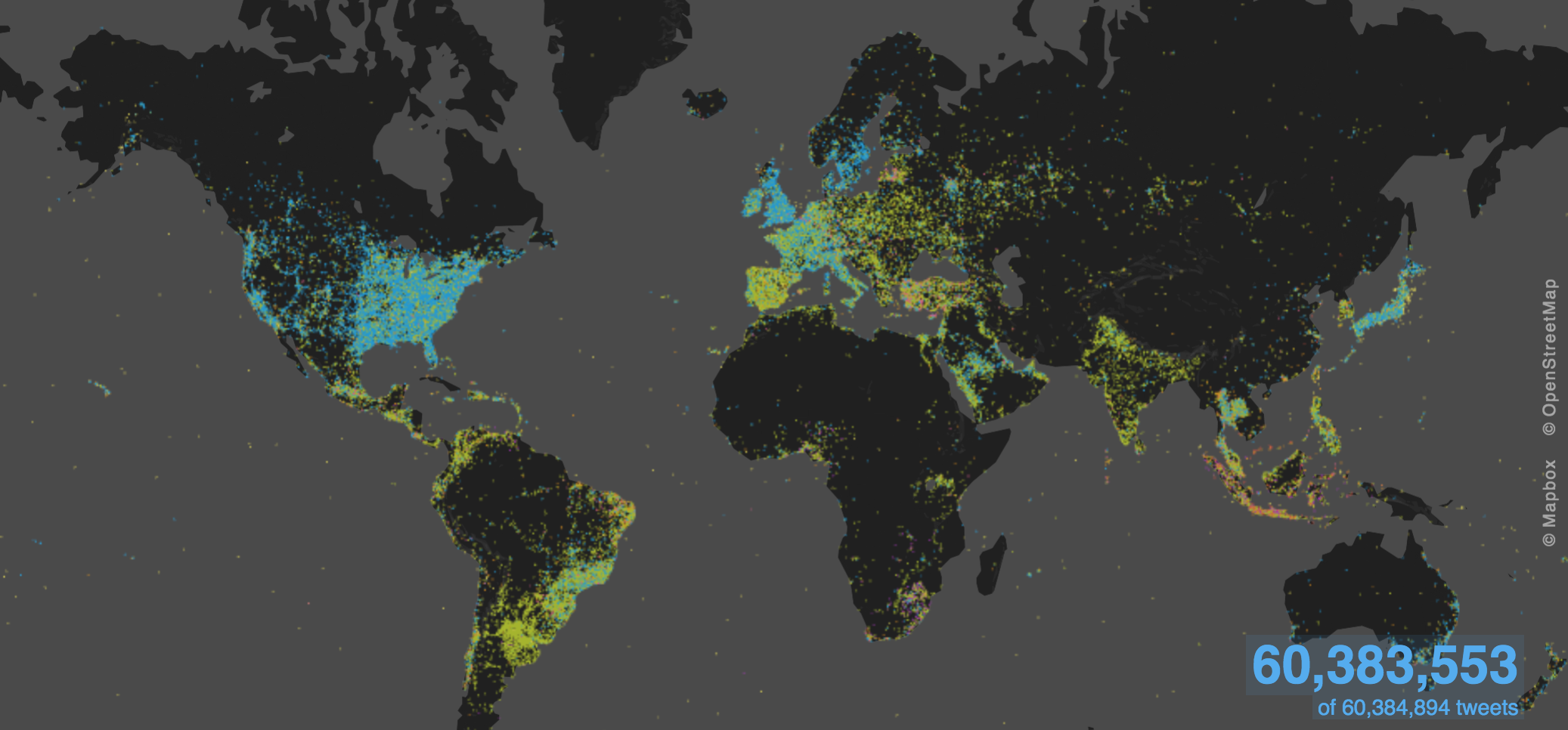
Figure 3: Pointmap of more than 60 million tweets colored by origin. Basemap courtesy of © Mapbox© OpenStreetMap

Shaderific

This declarative JSON format allows for a variety of data-driven rendering options. The power is in the scale functions, which, to keep with the speed theme, need to be fast. As these functions are render-specific, it made sense to write them into the render pipeline rather than doing some intermediate compute operation beforehand.

We therefore wrote a library of templatized scale functions in GLSL which are called during the vertex processing stage. As GLSL does not have the notion of templates, we designed our own “extension” of GLSL using a template format similar to that of C++.

The final shader source is dynamically written to true GLSL, compiled, and cached at runtime. As the scale references in the JSON are not likely to change frequently, only their parameters, runtime GLSL code generation and compilation is rare and therefore not a bottleneck.

Query-to-Render

The speed behind our query-to-render pipeline is the CUDA/GL interoperability API which allows us to write the query results directly to mapped GL buffers. No additional copy nor reduction operations are necessary thus allowing the result set to be sent off for immediate rendering. The GL buffers are pooled for use and can be resized when necessary.

Multi-GPU Rendering

In the case where the database requires multiple GPUs for storage, a subset of the query results are generated per GPU and rendered separately. We create the final image by copying the resulting color, depth, and any auxiliary buffers from each GPU to a 2D texture array on a primary GPU for compositing.

The copy method used is determined by the platform and windowing library configuration.

When configured to use X11/GLX on Linux, for example, we take advantage of the NV_copy_image OpenGL extension to copy buffers across contexts using the glXCopyImageSubDataNV() function. After the copy operation, we render the final image with a composite pass that samples the intermediate 2D texture array layer-by-layer, doing the alpha blending as we go.

We found this technique to be highly performant. We can render a 2000x1500 resolution, fully anti-aliased point map of a 2 billion-row dataset (limited to 2 million points) partitioned across 8 Nvidia Tesla K40s, in under 25ms.

Frontend Interactivity

On the frontend, our goal was to provide the most interactive data experience possible. This meant we needed the ability to extract specific data information when selecting or hovering over rendered data points. This required us to develop some form of a render-to-data operation.

We found that an optimal way to do this was by caching an auxiliary integer buffer on the backend that stores the data’s row ID per pixel. This buffer is attached to the framebuffer as an additional color attachment and is updated in the fragment shader at render time.

In the case where multiple data points overlap, the final ID at a pixel is determined by the depth test function; the last data rendered at a pixel wins.

This made a direct 1-to-1 correlation between render and data, but required a GPU to CPU transfer of the buffer post-render for caching. This was done asynchronously by using a pixel buffer object bound to OpenGL’s GLPIXELPACK_BUFFER binding point. This helped keep frame rates high, but still allow for quick per-pixel data lookups when necessary. To help resolve the hits at pixels near primitive boundaries, a Gaussian-weighted kernel is applied to the pixel's neighborhood. We found that a 5x5 neighborhood provided a sufficiently interactive experience.

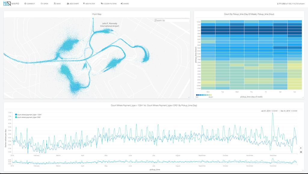
Figure 4: Visualization of taxi patterns at JFK airport. Basemap courtesy of © Mapbox © OpenStreetMap

Summary

The parallel power of GPUs present opportunities to create truly distinctive visual experiences with datasets that were once considered to be too large to render in real-time. To achieve success with billion plus row datasets is not a straightforward exercise and requires careful consideration of what techniques are suited for which tasks. The outcome is the ability to interact in realtime with massive datasets in a unique, hybrid visualization framework.

If you are interested in learning more about our technology, please engage with our demonstrations or reach out to us at info@mapd.com. We are hiring as well so please look at our openings on the company page. If you don't see a role, please don't hesitate to drop us a note a jobs@mapd.com.